I enjoy doing experiments with radio frequency stuff and this year I've built several antennas for receiving shortwave radio signals. One question I'd like to answer is which antenna is better. Evaluating the performance of an antenna usually requires expensive equipment and a dedicated laboratory environment. But I figured if I just want to compare two antennas I can get away with a less sophisticated test environment.

Setting up a test environment

In order to compare two antennas, I needed to use them to receive the same frequency and record each signal so that they can somehow be compared. There are numerous powerful shortwave transmitters in the United States such as WBCQ & WWV. A common technique is to switch between the two antennas and compare the apparent signal strength shown on a single receiver's S-Meter. While this gives an immediate comparison, it is only a single data point.

To get a better comparison between my two antennas I wanted to gather more data points. This meant I needed the process to be automated as well. In recent years amateur radio has seen an increase in the popularity of digital modes used on the shortwave bands. One of the most popular modes presently is FT8. This mode is supported by the WSJT-X software, which generally interfaces to a radio transceiver by using the sound card of a computer connected to the microphone and speaker of the radio. If you listen to the audio signal broadcast by most digital modes they sound like a series of tones. But each tone encodes some portion of the data and can be decoded by the software to recover the original message.

The utility of this for me is that I can leave multiple radios running with one connected to each antenna and run WSJT-X to gather a log of the received signals. This process would be completely impractical with non-digital signals such as voice or morse code. There is no way I could operate two radios simultaneously for days on end.

Each time WSJT-X receives a signal it writes it into a logfile, with each line looking like this

200817_193230    14.074 Rx FT8    -20  0.2 2171 CQ KW4SP EM64

The fields on each line are

1. UTC timestamp
2. Frequency in MHz.
3. The direction of the signal, always "Rx" for receive in this experiment
4. The digital mode in use, always "FT8" for this experiment
5. The signal level relative to the noise
6. Time offset
7. The frequency offset
8. The original message sent by the transmitting station

The most helpful values here are field 5 and 8. Field 5 is the signal-to-noise ratio given in units of decibels. This is a relative measure of signal strength, with higher being better. Field 8 is whatever message the transmitting station decided to send. For digital modes like FT-8 the format is largely standardized. In the case of the message "CQ KW4SP EM64" it means the station with callsign "KW4SP" is calling any station that wants to respond and is transmitting from the geographical location "EM64" as indicated by the Maidenhead Locator System. This means I can easily compute the distance to the transmitter.

So at this point I had come up with a way to gather data which I could later compare. This is only really practical because on a daily basis 1000s of radio amateur operators use FT8 on a small number of radio frequencies. This means in a single night I can easily record 100s of signals from my location. FT8 wasn't intended to be used to evaluate the performance of a receiver, but it works well enough for what I want to do.

The antennas

I have two antennas I want to compare in my test. I'll show both of them here, but I'm not going to try and explain much about them. Antenna theory is a bit out of my depth and there are plenty of good resources on the internet already. In the same manner this article does not contain long explanations of radio theory but does include links to the relevant Wikipedia article.

The inverted "L" antenna

The first antenna is a called an inverted "L". In my case it is constructed from a piece of copper coated wire that is suspended in the air. The shape it makes is like an upside down "L" character, hence the name.

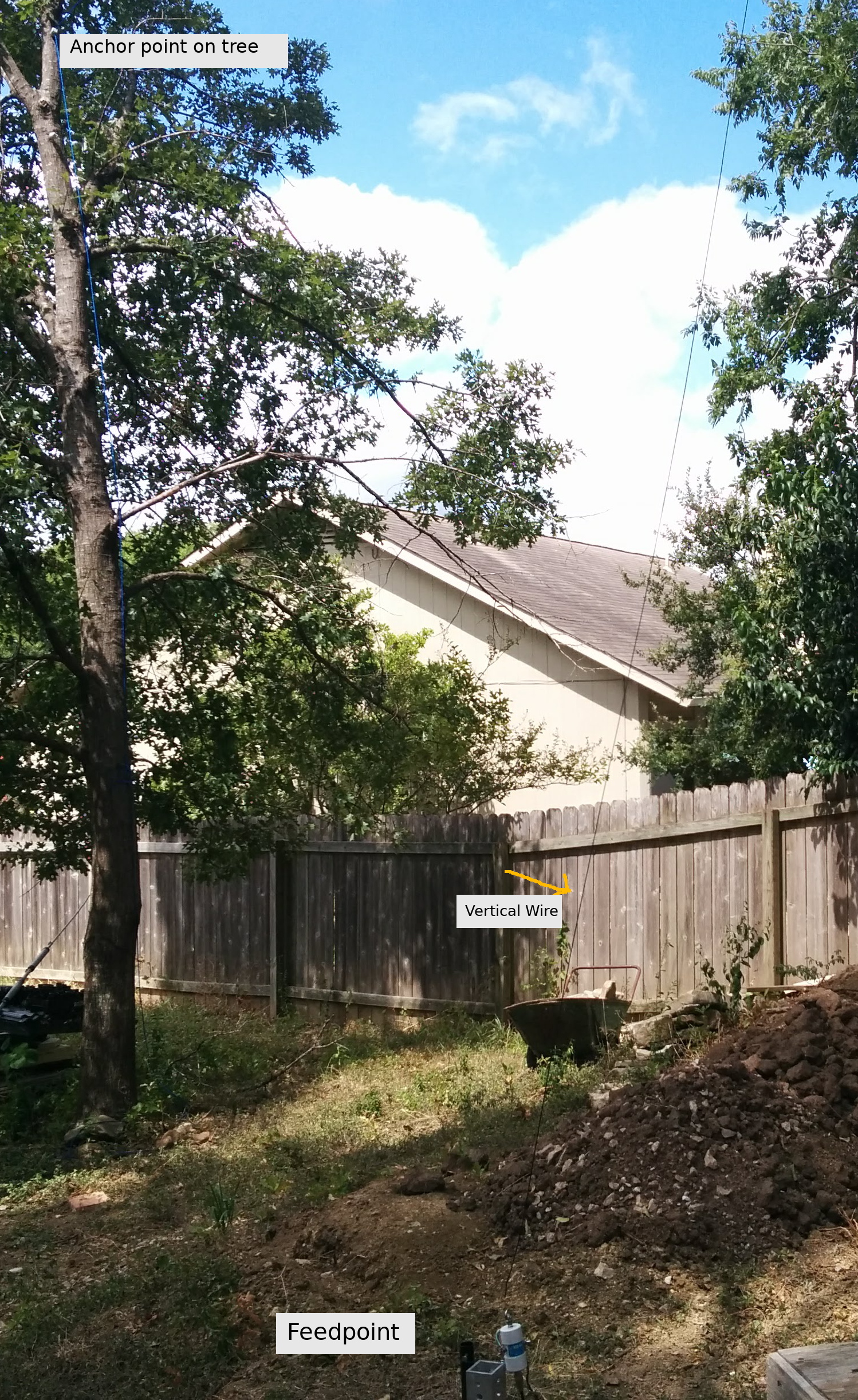
The antenna is constructed by anchoring it to a tree and another point overhead (not visible)

This type of antenna is designed to work on a single frequency and in my case I optimized it for a frequency of 7.050 MHz. This corresponds to the "40 meter" amateur band in the United States. The simplicity of construction means it is one of the first types of antennas many people built for shortwave radio reception. One important remark here is that although this antenna is designed to work on 7.050 MHz it still receives all frequencies. It just doesn't receive other frequencies as well.

If you'd like to know more about this antenna there is an extremely detailed explanation here.

T3FD antenna

The other antenna I built is called a "Terminated 3-Element Folded Dipole" or "T3FD" for short. This type of antenna was designed some time in the first half of the 20th century. My first exposure to this antenna was this website.

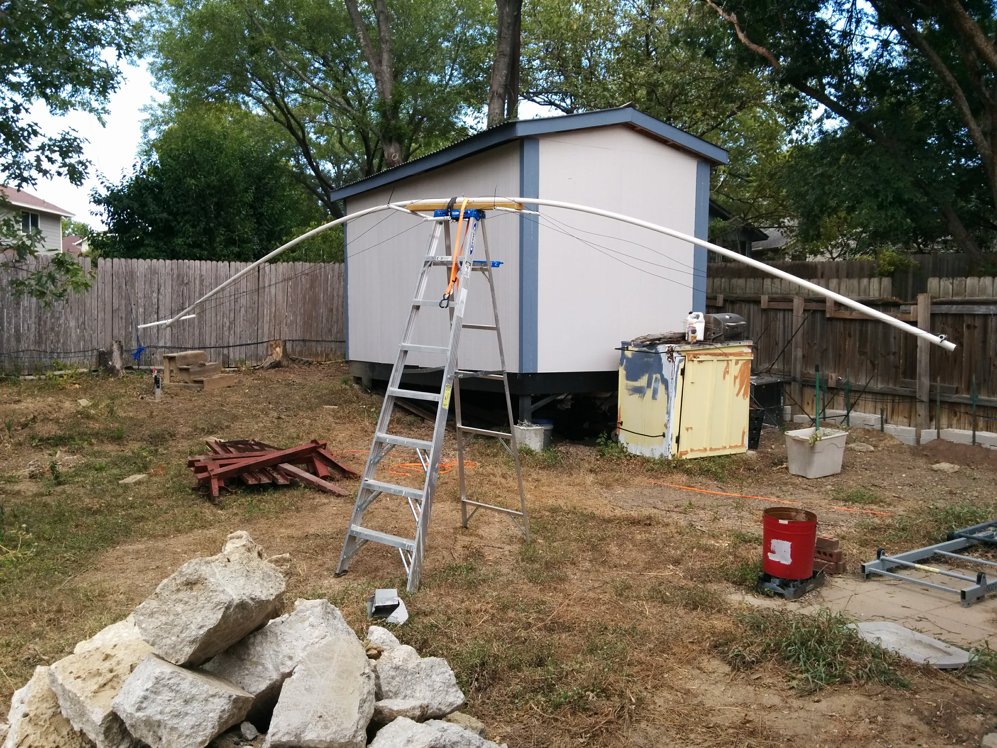
This is how the antenna was actually built. Using PVC pipes for supports works but it does sag under its own weight.

The advantage of this antenna is it considered "broadband" in that it can receive a wide range of frequencies equally well. One obvious difference of this antenna is that it is oriented horizontally. This is actually more common that a vertically oriented antenna.

I need to point out here that my construction of this antenna is massively different than what most people specify. In most cases the total length of a T3FD is given as 90 feet. Mine is only 20 ft long overall. It's also sitting about 8.5 feet off the ground, whereas the ideal mounting should be much higher in the air. In summary, this antenna is significantly different from what most people call a "T3FD" but does share the same construction charateristics.

The radio hardware

In order to receive shortwave radio you need some sort radio receiver. Such devices are typically expensive, but the RTL SDR has changed all of that. This device is a USB adapter that allows your computer to function as a radio receiver. It has significant drawbacks, but given its low cost is an excellent value.

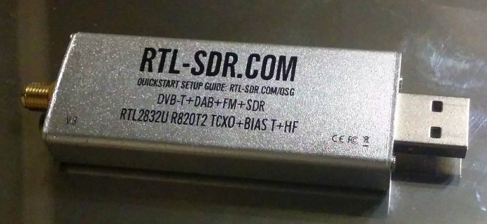
This affordable dongle converts RF signals into digital measurements

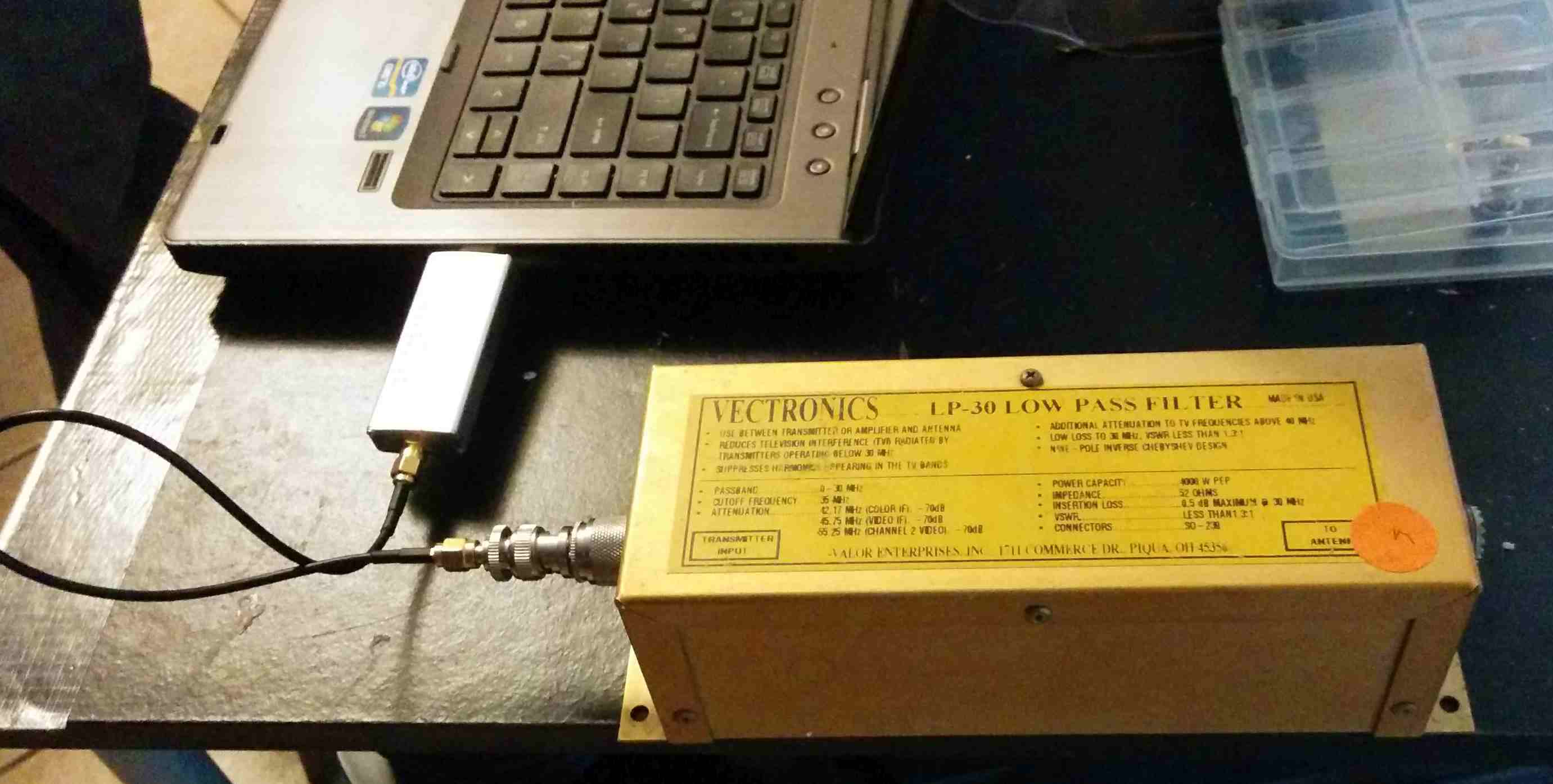
In my case I used two RTL-SDR receivers each paired with a shortwave radio filter. The purpose of this filter is to reject radio signals with a frequency higher than 30 Mhz. Using this filter tends to improve the sensitivity of the RTL-SDR dongle. This is because in a city environment extremely strong signals from TV & FM broadcast tend to overload the device.

On Linux I use the RTL SDR with the GQRX software receiver. The other advantage to using this I don't have to have any cabling to connect a radio receiver and my laptop. I am able to have GQRX play the audio out of the normal soundcard and then tell WSJT-X that the input sound is the output device. This might sound seem a little weird, but this is well supported on all modern linux distributions using pulse audio.

Automating reception

Since at least one of the antennas I am testing should be able to receive signals over a wide range of frequencies, I wanted to gather data about reception on mulitple frequencies. To do this, I needed to automate switching the GQRX receiver and WSJT-X. GQRX already has a TCP interface for remote control and WSJT-X uses UDP for remote control. Neither piece of software supported all the functions I needed over the remote control interfaces, so I ended up modifying them and compiling my own custom builds. Both projects are C++, which I am reasonably confident with.

Since I had two receivers setup, I had two instances of WSJT-X and GQRX setup on separate PCs. Using Python I was able to start a coroutine responsible for setting the state of each piece of software. Each coroutine just listens on a asyncio.Queue for a new configuration and then sends the appropriate commands across the network. I like this design pattern because it gives each coroutine a single responsiblity.

Controlling GQRX

The coroutine for controlling a GQRX instance just starts up, connects a TCP socket, then sends the appropriate commands to other end. This is all done inside of a loop. If there is an exception, the coroutine sleeps for a while then reconnects and applies the same commands. This is a simple way to deal with the fact network connections can be temporarily interrupted. In my case I was using WiFi, so it's likely that the connection would need to be re-established.

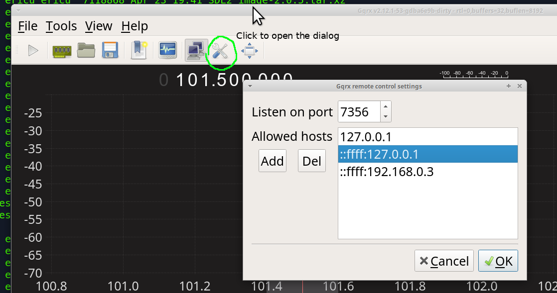
There was one unusual issue with GQRX. The remote control interface is secured by means of listing the allowed IP addresses. This isn't actually very good security I'd like to point out. In any case, I struggled to get it to allow me to connect remotely. It turns out although my home network is using IPv4, the IP address needs to specified in IPv6 notation. So to allow a remote connection from 192.168.0.3 you need to actually enter a remote IP of ::ffff:192.168.0.3.

Controlling WSJT-X

The coroutine for controlling WSJT-X is a bit different. The remote control interface for WSJT-X is rather unique. It uses UDP, but in the software you configure the a hostname and port as the destination. It sends packets with information about signals received and the current state of the program at regular intervals. You send UDP packets back to the originating port to issue commands to WSJT-X. The structure of all the messages is documented in the file Network/NetworkMessage.hpp in the git repository. Each time a UDP packet is received by my Python script, it saves the remote IP and port. Since my Python script could not be sure to receive the first packet before the first command to set the frequency of WSJT-X, it needs to apply the current configuration each time the remote IP & port changes. When this happens it usually means WSJT-X was restarted and needs to be configured again. Due to this there is a slight delay from the time the script is first started to the first time it can configure WSJT-X. However, this delay only a few seconds and isn't really significant since I collected data for days.

The first problem I ran into was WSJT-X seemed to simply stop communicating over UDP. On the machine running WSJT-X I would find it displaying this error.

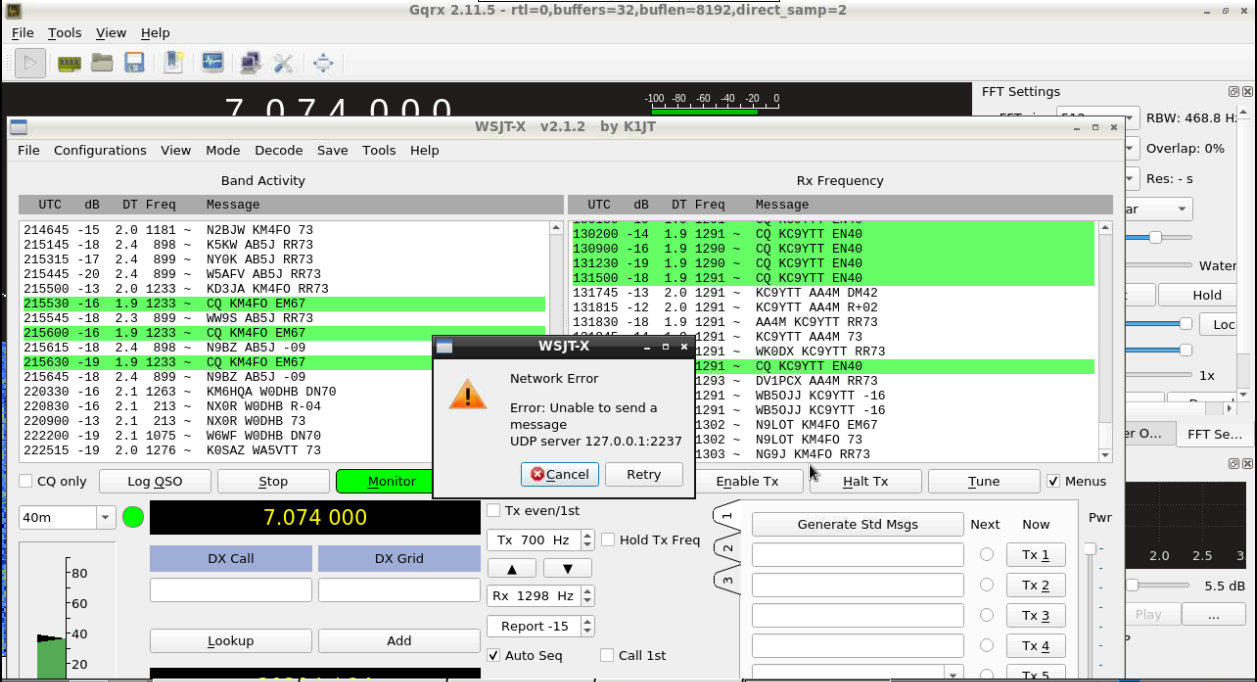
This error message was about as helpful as a dialog box saying "Critical error!". If I clicked "Retry" everything immediately went back to normal. The only thing I could guess was that for some reason the network interface was temporarily unable to send UDP packets. I was able to track down this dialog box to a single C++ member function

void MainWindow::networkError (QString const& e)
{
  if (m_splash && m_splash->isVisible ()) m_splash->hide ();
  if (MessageBox::Retry == MessageBox::warning_message (this, tr ("Network Error")
                                                        , tr ("Error: %1\nUDP server %2:%3")
                                                        .arg (e)
                                                        .arg (m_config.udp_server_name ())
                                                        .arg (m_config.udp_server_port ())
                                                        , QString {}
                                                        , MessageBox::Cancel | MessageBox::Retry
                                                        , MessageBox::Cancel))
    {
      // retry server lookup
      m_messageClient->set_server (m_config.udp_server_name ());
    }
}

Since clicking "Retry" seemed to make everything go back to normal, I decided to edit the code to skip the dialog box entirely like this

void MainWindow::networkError (QString const& e)
{
  QString x = e; // 'use' the argument
  if (m_splash && m_splash->isVisible ()) m_splash->hide ();
  // retry server lookup
  m_messageClient->set_server (m_config.udp_server_name ());

}

I'm sure the error still happens, but it probably means that just a single UDP packet is lost. With UDP this is expected anyways.

I tried several times to use WSJT-X running on an Raspberry Pi 3. It takes an extremely long time to compile, but does work. If I just left it running it seemed fine. But using the remote control UDP interface during periods of high traffic would lead to the user interface becoming unresponsive and the process consuming 100% of a CPU core. WSJT-X is written using Qt5 extensively. I am guessing there is some sort of race condition that leads to this happening. I did not want to spend time trying to track down the race condition, so I tried running everything on x86-64 computers. The problem did not happen there. My conclusion is this a platform specific bug, possibly caused by differences in the assembly instructions emitted by the compiler.

Receive frequencies

With my script to automate everything working, the frequencies I chose to receive on are

1. 3.573 MHz
2. 7.074 MHz
3. 10.136 MHz
4. 14.074 MHz

These are all standard frequencies used in the amateur radio bands for the FT-8 digital mode. At this point I let everything run for a number of days to collect data.

Comparing the log files

Once I had collected data I needed a way to compare both log files. I wrote a Python script that could take both files as input. The inverted "L" had recevied 65,212 signals whereas the T3FD antenna received 36,053 signals. So I needed to compare a total of around 100,000 datapoints. Since the log file is just text I used a regex to parse out each line and convert it into a Python object. I didn't want to try and hold 100,000 Python objects in memory so what I needed a way to store the objects on disk.

What I did was pickled each object using Python's built in pickle module. This turns the object into a bytestring that can be saved to disk. The length of this byte string is written first to disk as a 16 bit integer then the actual pickled object is written. This allows each object to read one at a time from the file. All this is stored in the a temporary file created using the tempfile module, so it disappears when the .close() method is called on the file object.

def write_object_sequence(fin, objs):
  for x in objs:
    pickled = pickle.dumps(x)
    header = struct.pack('>H', len(pickled))
    fin.write(header)
    fin.write(pickled)

def read_object_sequence(fin):
  fin.seek(0)
  while True:
    header = fin.read(2)
    if len(header) == 0:
      break
    data_len, = struct.unpack('>H', header)
    yield pickle.loads(fin.read(data_len))

These two Python functions implement this. The write_object_sequence function takes two arguments fin a file object & objs which is any Python object that can be iterated over. Each object is pickled one at a time. The struct module is used to convert the length of the pickled object into a byte string as well. Both are written into the file.

The read_object_sequence is able to do the opposite of the above. First, two bytes are read and passed back to the struct module to recover the length of the pickled object. Then, that many bytes are read from the file. The object is then unpickled by calling pickle.loads. Importantly, the yield function is used so that the objects are passed back to the caller one at a time. This means not every object in the file is read into memory at the same time.

This is a simple method for working with a large dataset on-disk without external dependencies.

Direct comparison

The first comparison I wanted to make was to look at the number of signals received by each antenna on an hourly basis. If one of the antennas does not receive many signals at all, then it is unlikely any other comparisons are going to be worthwhile. What I did was summed up the counts of signals on per-frequency basis for each antenna over all the hours in the dataset. I generated a different graph for each frequency. This was done by writing a single CSV file containing all the counts and a command file for Gnuplot that creates separate graphs as PNG files.

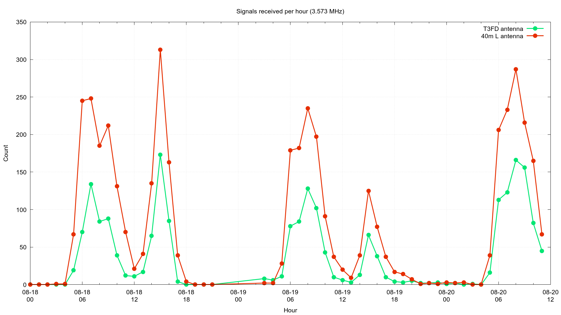
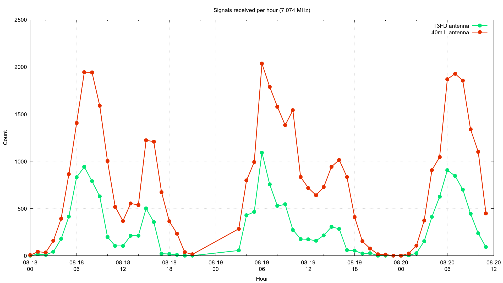
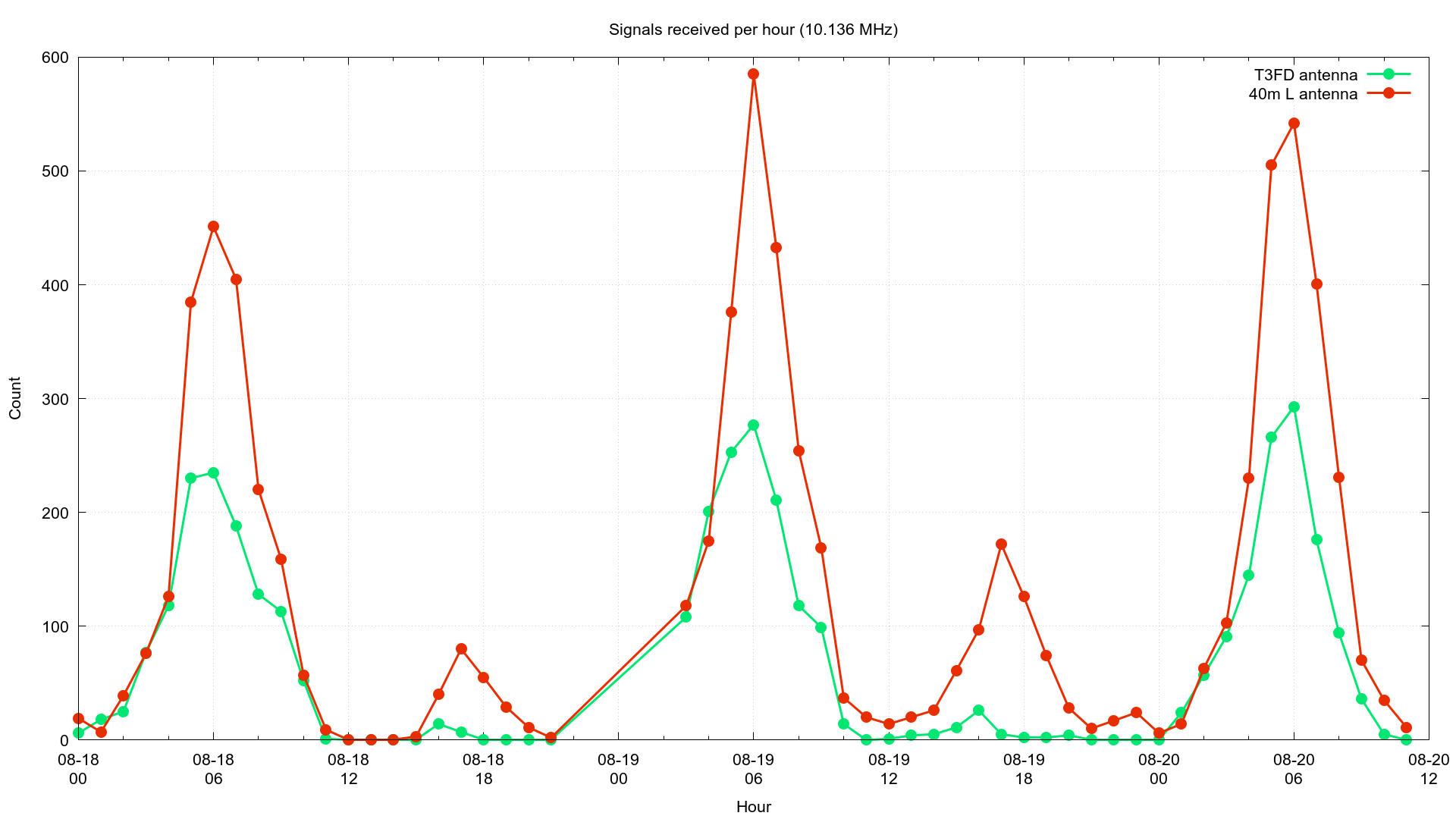
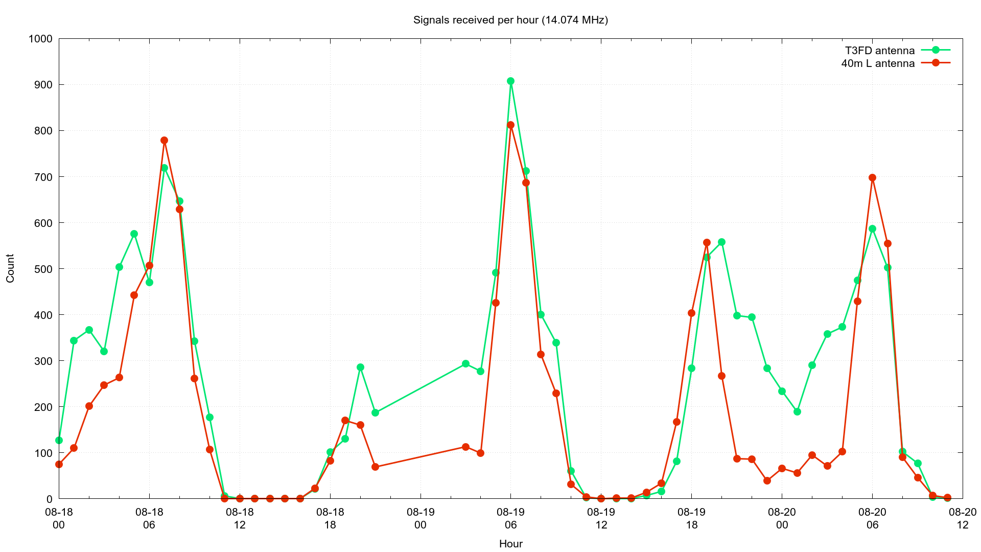
This shows that the inverted "L" receives about twice as many signals per hour as the T3FD antenna. But the T3FD still receives 100s of signals per hour, so there is enough data to compare the two antennas.

The other comparison I wanted to make was by using the Maidenhead Square locator included in some of the signals to determine the maximum distance of the received signal for each hour by each antenna. In order to do this I wound up using the maidenhead package to convert them into latitude & longitude. Once I had this I could use the pyproj package to compute the shortest distance from my location to the transmitter.

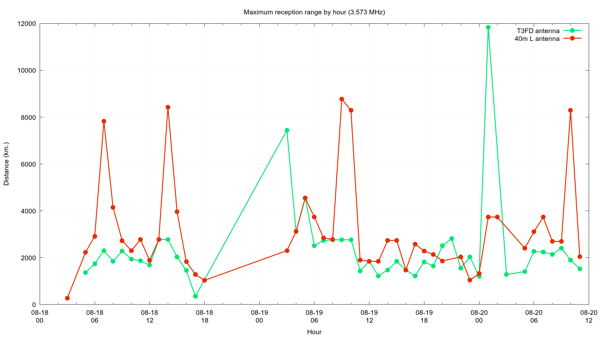
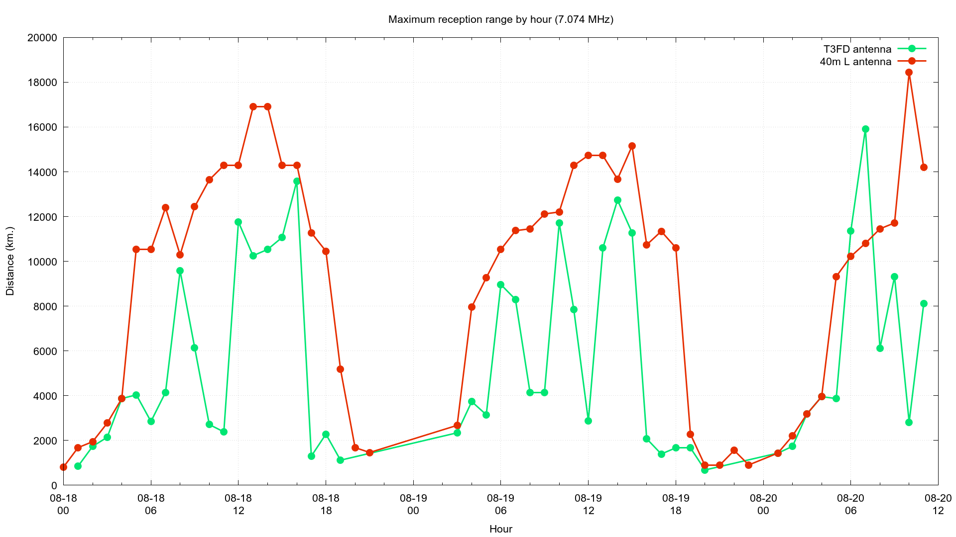
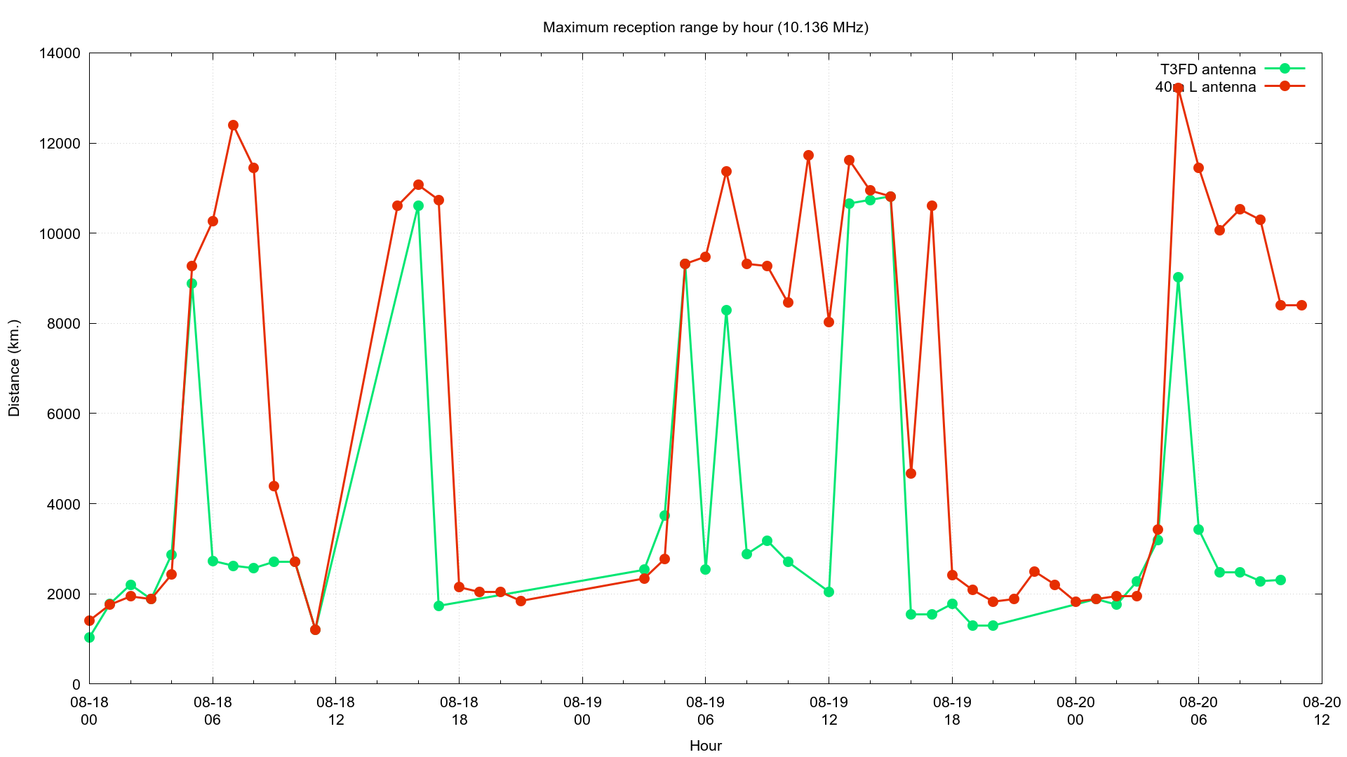
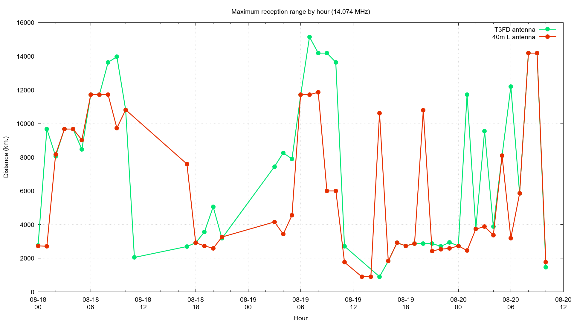
The conclusion that can be made is that the inverted "L" antenna has a distinct advantage at receiving far off signals. There is one hour on 3.583 MHz where the T3FD wins but I think that is just some sort of fluke.

The shortcoming of these comparisons is you can't make an objective statement about either antenna being "better". While a count of signals received is an interesting metric to compare, it doesn't tell the whole story. For example, even if two antennas receive an identical number of signals in a 1 hour period it is entirely possible that each antenna receives a different set of signals. The same can be said with respect to distance. Some antennas are actually optimized for receiving nearby signals, whereas others may be better at receiving far off signals.

Relative comparison

I wanted to make a direct numerical comparison between the two antennas. To do this, I needed to compare only signals which both antennas received. So to do this I needed to try and match each signal from one log file to another in the other log file. The obvious manner in which to do this is to try and use some unique key for each signal and put them into a Python dict. A unique key for each signal consists of

1. Timestamp
2. Frequency
3. Frequency offset
4. Message

The first problem with this is the Python dictionary would contain more than 10,000 entries even with my small dataset. This would probably fit into memory, but I decided to use the shelve module. The shelve module acts like a dictionary but values are stored as a pickled object on disk. This allows me to match up the data on disk rather than in memory.

The other issue is frequency offset. Radio receivers are not exact devices. Two seemingly identical radio receivers often report slightly different frequencies for the same signal due to environmental sensitivity, such as changes in temperature. The difference is small, usually less than 50 Hz. But this would be enough to cause signals not to match up. One option would be skip comparing the frequency offset entirely. But I didn't want to do that. My solution was to use a key consisting of timestamp, frequency, & message. I was able to override the Python __hash__ function and pass a tuple of the data so that each object with the same values had the same hash. This does introduce the possibility of collisions in the hash value, but this is solved by comparing the complete set of values for each signal after the grouping by hash is complete.

With all that taken into consider I came up with the following algorithm

1. Iterate over each file, storing each signal at the key for its hash in the shelve dictionary
2. Iterate over the shelve file one key at a time
3. Compare all the signals stored at that key, finding those signals which are received by both antennas
4. Compare the matched signals frequency offset and make sure the magnitude of the difference is less than 100 Hz

The actual structure I used for storing signals in the shelve used a nested structure of dictionaries and lists, shown here is an example

{
  "76ab": {
     "T3FD antenna" : [<Signal 1>, <Signal 2>],
     "L antenna" : [<Signal 3>, <Signal 4>]
  }
}

In the above example "76ab" is Python hash value of all the signals stored at this key. The shelve module requires that the keys be strings so each numerical hash is stored in it's hex representation. Stored at the key is a dictionary with two lists, one for each antenna. Since signals are stored by hash, it is possible for collisions to occur. This means otherwise unrelated signals are stored at the same key. Performing an actual comparison of the value in each stored signal prevents an other erroneous match from being made.

The performance of this implementation is superior to the obvious implementation of comparing each signal received by one antenna to all other signals received by another antenna. The complexity of such an obvious algorithm would be \(O(M*N)\) where \(M\) and \(N\) is the number of signals in each file. Instead, this just compares each signal to the other signals stored at the same key. This winds up being the same class of complexity but the quantity of signals in each list is much smaller. There is the added cost of the step to group the signals by key, but it still faster. This process of splitting the input into smaller groups then anlayzing each group on its own is basically the MapReduce algorithm. Usually this involves trying to perform both the map & reduce steps with as much parallelism as is possible. I did not do any of this in parallel because a single threaded Python program is more than fast enough for me.

For each pair of matched signals I computed the difference in the signal-to-noise ratio between each reception report. This number is actually a valid metric of comparative performance. Since many thousands of signals were recevied by both antenna, I averaged these values for each hour and then plotted the average. Computing the average difference produces just one dataset for each frequency, so I was able to make a single color coded graph showing these differences.

I chose to exclude any signal received from a distance of less than 175 kilometers. This is done because at such a short range almost any conductive piece of metal is good enough to receive these signals. It isn't a useful comparison to measure signals from such nearby transmitters.

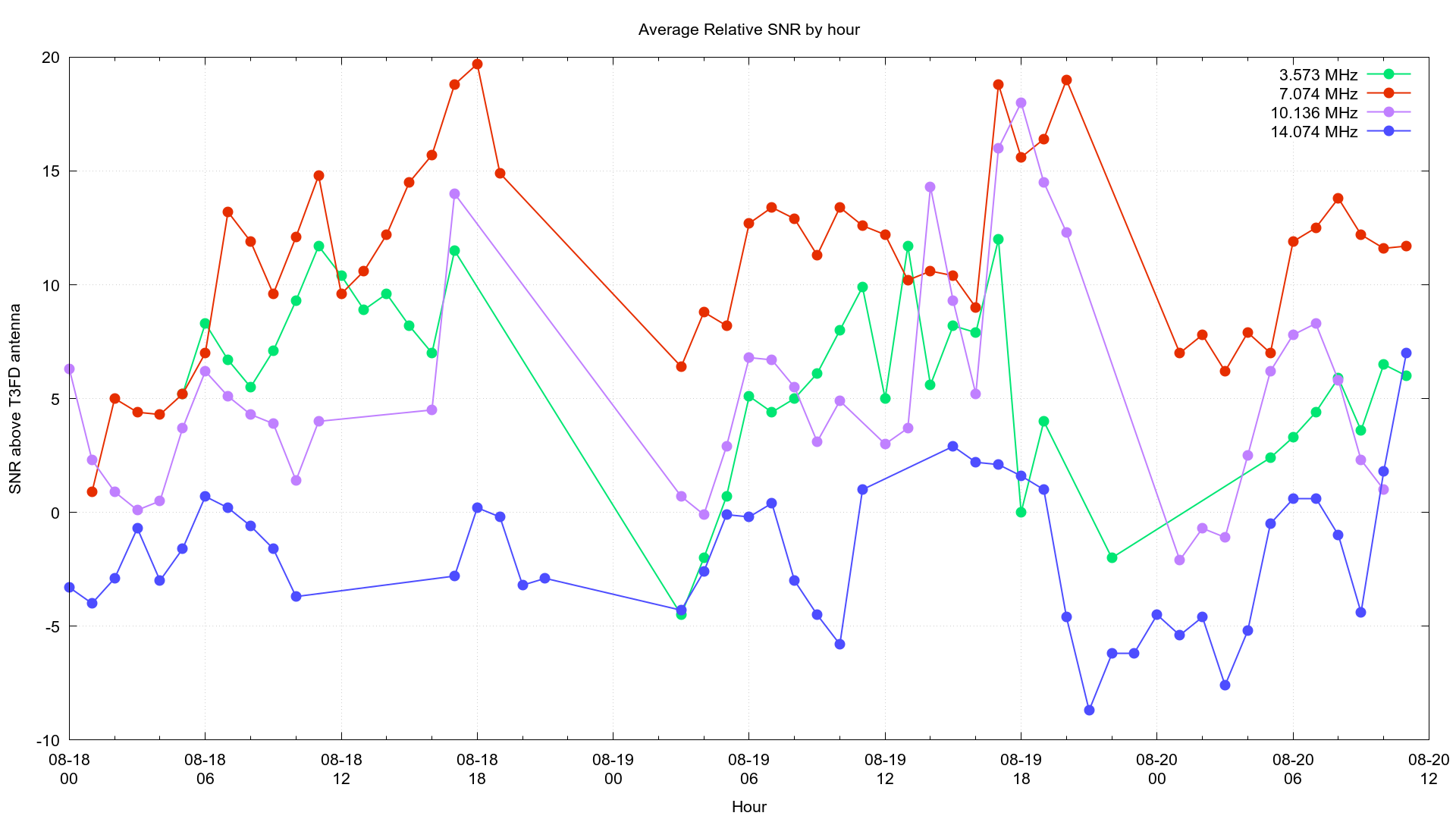
This comparison shows that the inverted "L" outperforms the T3FD for most of the frequencies tested. The blue line is for 14.074 MHz and at this the average value is usually negative. This means the average signal-to-noise ratio of signals on that band is in fact higher on the T3FD. The reason for this is that the inverted "L" antenna is designed to operate on 7.074 MHz and has a physical wavelength that is twice that of an ideal antenna for 14.074 MHz. This length of wire turns out to be an exceptionally poor antenna.

This conclusion is useful, but also has the shortcoming of only being able to make a comparison in the case which both antennas receive the same signal. For antennas with nearly identical performance it would likely be useful, albeit uninteresting. In my case it's pretty obvious that the antennas significantly differ in performance.

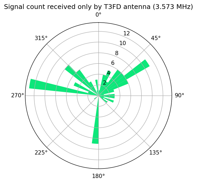
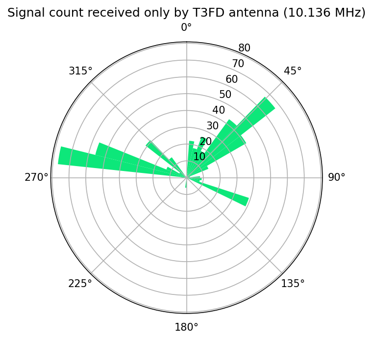
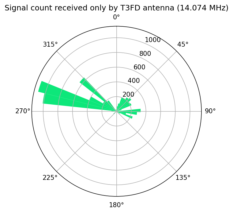
Differential comparison by signal heading

The last comparison I chose to make was to compare signals received only by one antenna. I call this the differential comparison. This has the advantage of being the inverse of the "Relative comparison", so the logic is identical except only signals with no match are selected. Instead of grouping each signal based off the time received I grouped them by heading. I divided the 360 degrees of the compass into 45 divisions each 8 degrees wide. I was able to use to pyproj to identify the heading from my location to each transmitting station. If I didn't receive the grid square for a transmitter, I simply ignored that signal in the analysis.

Using the heading is based off the assumption that the shortest path (a Great Circle) is how the signal reached my destination. This isn't strictly true, but there is no other way to get the heading without using huge pieces of equipment. One interesting thing I noticed is that pyproj always gives a result in the range (-180.0, 180.0) which corresponds to a heading that is either left or right of north. I added 360 to each value to convert to the more commonly used compass heading.

Plotting with matlib

With the data sorted out by heading for each antenna, I needed some way to display it. I like using Gnuplot for most of my plotting but it isn't very good at making a polar plots. So I installed matplotlib which I have used in past projects. Making a single polar plot with matplotlib is easy as shown here

import matplotlib.pyplot as plt

# These are the variables that would contain the data to be plotted
heights = [...] # Array of count values
x_coords_radians = [...] # Positions to plot each "height" at around the circle
colors = [...] # Array of colors for each bar
widths_radians = [...] # Width of each bar

title = "Signal count received only by %s (%s MHz)" % (cat, freq_human,)
ax = plt.subplot(111, projection = 'polar', title = title)
ax.set_title(title)

ax.set_theta_zero_location('N') # 0 degrees is straight up
ax.set_theta_direction(-1) # Increasing in the clockwise direction
label = "Count"
ax.bar(x_coords_radians, heights, color = colors, width = widths_radians, bottom = 0.0, alpha = 0.95, label = label)
fname = 'differential_count_by_heading_%s_%dHz.png' % (cat, freq,)
plt.savefig(fname, format = 'png', dpi = 150, bbox_inches = 'tight')

After settting the projection to polar, you actually just make a standard bar chart. Except with the polar projection the bars radiate from a single point at the center. I had to make "up" the North (0 degrees) location and make the values increase clockwise.

Calling ax.bar is where the data is passed in. Most examples pass in a numpy object, but passing a regular Python list works as well.

The value x_coords_radians is the divisions of the polar plot. Since I grouped my data into evenly spaced headings, this is always a series of numbers 0, 8.0/(180*math.pi), 16.0/(180*math.pi) increasing until 352.0/(180*math.pi) is reached. This has to be given in radians, not in degrees.

The heights is an array of numbers that indicate how tall each bar is. For a polar plot, this is the distance from the center. Matplotlib is smart enough to automatically scale the plot so all data is visible.

The colors is the colors of each bar, I specified the same color for each bar. The value width_radians is just the width of my divisions so 8.0/(180*math.pi) repeated. The length of x_coord_radians, heights, colors, & widths_radians should all be identical. Even if you want to skip drawing a region you must include a height value of 0 in the heights array for that position.

The result

This comparison produces a total of 8 graphs, one for each antenna on four frequencies. The first pair to compare is for 7.074 MHz.

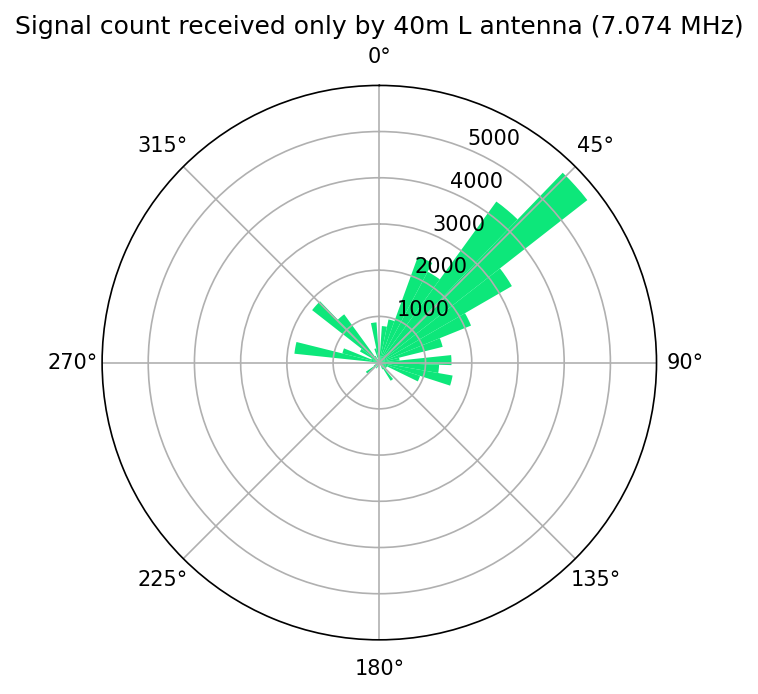
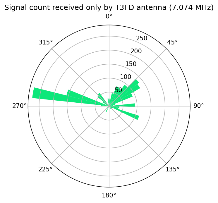
Looking at these two plots we can see the inverted "L" antenna received over 5000 signals from a heading of 45 degrees that were not received by the T3FD. This heading corresponds to the American Northeast as well as parts of Europe, so this isn't surprising. On this frequency I expect the inverted "L" to outperform the T3FD in all regards. What I found interesting about this is that T3FD received over 250 signals from a heading of about 278 degrees that were not received by the inverted "L". This is an unexpected result. I don't have a conclusive explanation for this. But the top section of the inverted "L" that is horizontal points almost due west. It is possible that the antenna is actually "deaf" in that direction and does not receive very well.

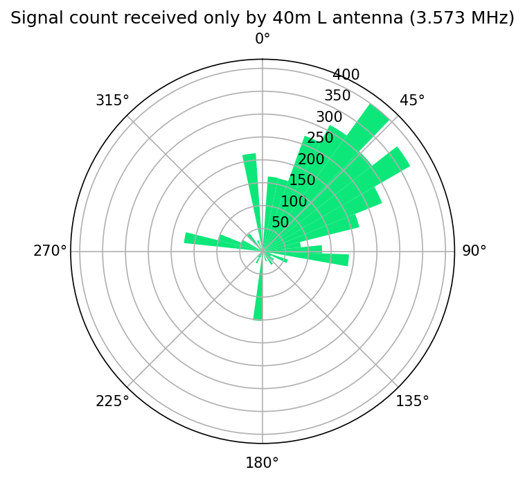
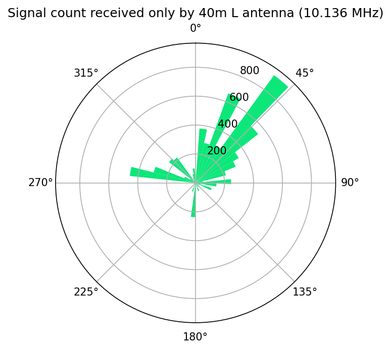
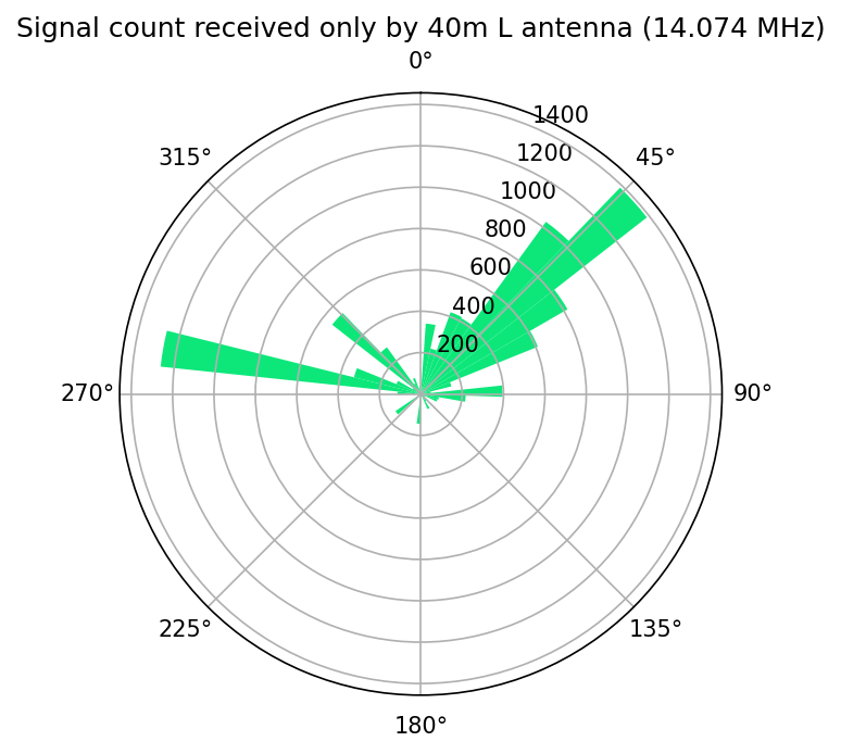
These plots show the remaining comparisons.

Conclusion

The main lesson I learned from this is that my inverted "L" antenna does not receive signals from a heading of West very well. I also learned that the T3FD antenna I constructed works pretty well given its relatively small size. I was able to make some direct comparison between both antennas, showing me that the inverted "L" antenna is much more sensitive at least on 7.074 MHz.

I also got to learn more about controlling GQRX & WSJT-x remotely. I plan to use both pieces of software more for later projects, so this should come in useful.

The Python shelve module is pretty cool, I am surprised I have not used it yet! If you need to store objects in a persistent key-value store then I highly recommend it.

Code

Modified version of GQRX: GQRX fork on my Github

Modified version of WSJT-X: WSJT-X fork on my Github

Python code to compare both log files: antenna_rx_difference on Github

Dataset

This is the original dataset containing both log files that were generated from the WSJT-X. Feel free to reproduce the graphs above or do other analysis on it.