In October of 2019, AWS introduced AZ64 compression encoding and made this claim

Compared to ZSTD encoding, AZ64 consumed 5–10% less storage, and was 70% faster.

The "compression encoding" of a column in a Redshift table is what determines how it is stored. There are a bunch of different options with each one offering a different type of compression. AZ64 is the most recent one to be added and is a "a proprietary compression encoding". Presumably since this was custom designed by AWS it should exceed the performance of more general purpose compression algorithms.

The team I work with at my employer uses AWS Redshift to store and query time series data. We had settled on ZSTD encoding for most of our columns. I have previously done some performance tuning to try and identify ways to make the queries faster, but did not find much in the way of gains. If using AZ64 is anywhere near 70% faster it would absolutely be worth switching to. I decided to benchmark AZ64 vs. ZSTD.

Test table structure

In order to run a test comparing AZ64 & ZSTD I needed to build a dataset in an AWS Redshift cluster that was similar to our production dataset.

Our table structure looks something like this

1. Time ID - A timestamp stored as an integer, RAW encoding
2. Customer ID - A customer ID stored as an integer, RAW encoding
3. Dimension columns - Columns which identify the type of the data point as integers, ZSTD encoding
4. Value columns - Columns storing the acual values which are always counts, ZSTD encoding

You can think of the Time ID, Customer ID, and Dimension columns being the "key" into the database. This describes what customer had what kind of event at a specific time. The value columns indicate how many times the type of event occurred. The values stored in the dimension columns are enumerations.

Redshift also has the concept of distribution style which tells Redshift how to shard each table. For our distribution style, we use the Time ID column as a key and a compound sort key based off the Customer ID and the Time ID. We also split the time series data across multiple tables as indicated in the AWS Redshift documentation.

The data stream of events used to build this data can come in with any ordering. So it is expected for rows to share the same "key". In order to present this data to an end user we run a query like this

SELECT time_id, dim_col1, dim_col2, SUM(value_col1), SUM(value_col2) FROM data_table WHERE customer_id = 33 
WHERE time_id >= 1000 and time_id < 2500
GROUP BY (dim_col1, dim_col2) 
ORDER BY (time_id, dim_col1, dim_col1)
LIMIT 100;

This type of query means that no matters how many rows in the table store information for a given "key", the user only sees one row since they are all combined using the SUM operator.

This is the typical way to store time series data in a Redshift table. In order to populate rows into each table I used a Ruby script to randomly generate rows of data for each customer. Some test customers have many rows in the table, some have few.

Test steps

I created two sets of tables in order to test each encoding side by side in the same Redshift cluster. My test cluster consisted of two dc2.8xlarge type nodes. One set of tables uses the ZSTD encoding. The other set of tables uses the new AZ64 encoding.

The steps for this were as follows

1. Create the set of tables
2. Run TRUNCATE TABLE on each table
3. Use COPY ... FROM s3 statements to load data files from S3 into each table, specifying COMPUPDATE OFF
4. Run VACUUM FULL on each table
5. Run ANALYZE on each table

Specifying COMPUPDATE OFF is required to prevent AWS from changing the compression encoding on a column for you automatically.

Running VACUUM FULL allows the table to be sorted by Redshift.

At this point the only remaining thing was to run a bunch of test queries on each table and compare the execution time. I had a list of Customer IDs I had generated data for and I also knew the time range for which data existed. Knowing this I randomly generated queries which covered both short and long time ranges. Each query was run on a fresh connection established to the AWS Redshift cluster.

Test results & conclusion

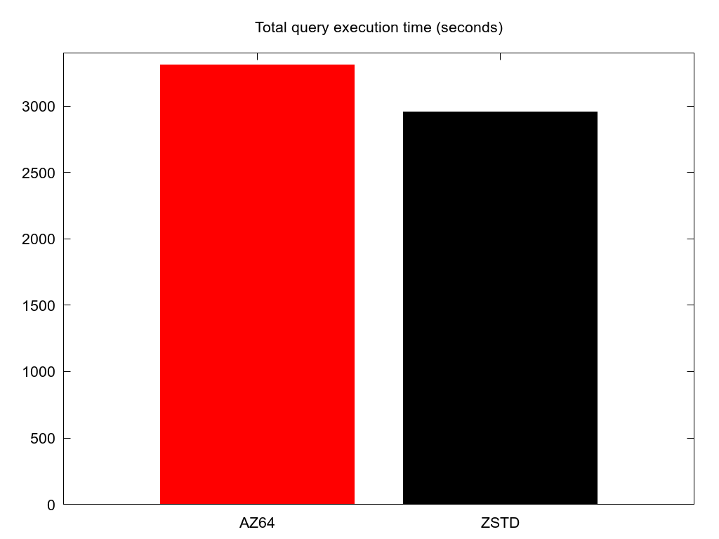
I ran a total of 240 queries for both types of compression encoding. I summed the execution time across all of them.

Unforuntately for AZ64, it took 3307 seconds while ZSTD only took 2953 seconds. This is an increase in execution time of 11.9%. I was at least hoping that AZ64 would be equivalent performance to ZSTD.

There is also the possiblity that for some subset of queries AZ64 is actually faster. I looked through the dataset and found nothing to indicate this. There are some samples where AZ64 was faster, but it is almost always when the query execution time is less than 1 second. This is just measurement error, as Redshift has some sort of floor on execution time even for trivial queries. Also, I'm not interested in trying to speedup queries already taking less than 1 second.

I also graphed the worst case execution times for several of my simulated customers. These queries are for customers with the largest number of rows in the tables. This shows the comparative amount of time spent querying the tables for a given customer using AZ64 vs. ZSTD.

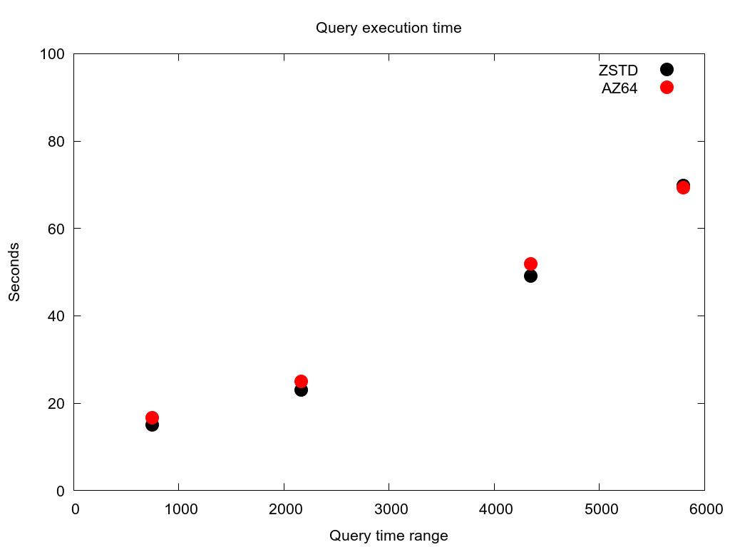
Large customer #1

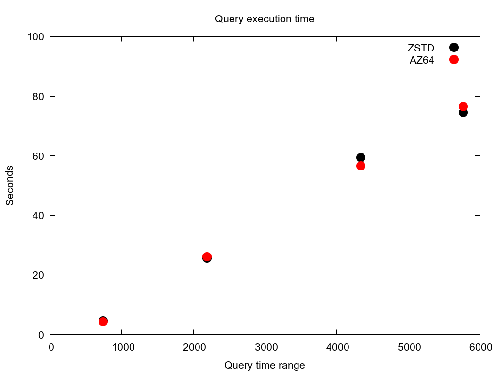
Large customer #2

For each case there is no clear winner. They both follow the same general slope, indicating that the column encoding is probably not the largest bottleneck anyways. But AZ64 is clearly not a real improvement over ZSTD in any way I could measure. So my conclusion is that for my use case not only is AZ64 not 70% faster, it is actually slower. I could find no information about how AWS came up with this 70% figure or what their benchmarking methods were.