Sniffing out probes part 2

In a previous blog post, I detailed how I began capturing WiFi probes from the roadway in front of my residence. Now that I have collected a decent amount of data, I decided it was time to do some analysis on it.

Flawed data capture

Whenever I wrote the code to gather probes, I made the assumption that most stations would be sending out directed probes (for a specific SSID) rather than undirected probes (for any SSID). I did not originally record undirected probes. When I started looking at the data, it was obvious that I was discarding a large amount of potentially interesting data. I had observed 9450 unique stations, but only 1947 of those sent directed probes. By discarding the undirected probes, I was only recording probes from 20% of the stations that I otherwise could be.

As a result, I've modified the capture script to record undirected probes from stations. I'm now recording that into a separate database from the original database.

I opted to go ahead and do some analysis now on the existing data set. All of the graphs and data presented here are gathered from the original data set.

The original idea

When I started this I thought that I would be able to analyze the data and notice patterns in the observations of certain stations. So far I have not been able to do this. The reason is only a percentage of stations are observed sending probes more than once.

As this chart shows, less than half of stations are observed more than once. If you are looking for patterns in a specific stations activity, this means that less than half of the dataset is of interest.

Analysis

Overall I observed 32022 probes from 1947 unique stations.

Background subtraction

The same probe is recorded only once in a five-minute period. As a result the recored number of probes for some stations is much lower than the real world number of probes. This means that a station probing for some SSID can be recorded no more than 288 times in a day. This is necessary because in any area there are some number of stations that are always there. Most of those stations are associated with an access point and are not actively sending probes, so the capture script does not record them. However, some fraction of them are not associated and may be constantly probing. Common sources of such probes are things like WiFi capable printers which have never been set up. The five-minute period limit stops those stations from simply flooding the database with records and quickly filling it up. Since I am interested in observing the probes only from the traffic in front of my house, these stations are deemed background noise. I don't intend to count them in the analyzed data.

The upside to using this five minute period is that any station persisently observed should have an inter-observation period average of five minutes. The inter-observation period is the time between which a station is observed probing for the same SSID. This period should be a normal distribution centered around an average value of five minutes.

The distribution of the inter-observation period for a non-background station is unknown at this point in time. However, even if it is also a normal distribution it should not be centered around five minutes.

For each combination of station and SSID I calculated the inter-observation periods. Furthermore, any station that did not have at least 144 independent observation events (one hours worth) I decided it could not be a background station. Then, I calculated the 95% confidence interval for the inter-observation period. If the value five minutes lies within this interval, I conclude that the station is a background station. That station is excluded from the final results.

There is a good chance that this analysis make somes statistical assumption that is untrue. However, starting from the idea that a background station should always be observed and that a station in a vehicle is observed infrequently then it can be concluded that background stations should make up a disproportionate amount of the observed probes. The statistical method I presented identifies stations in agreement with this idea. I identified 12 stations which were reponsible for 50.95% of the observed probes.

Probes by day of the week

The first thing I decided to look at was the number of probes per day of the week.

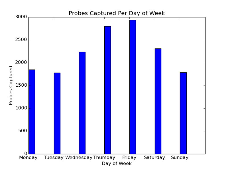
This graph is not particularly interesting. There are more probes recorded on Friday than any other day of the week. This lines up with the idea that more people are out doing things on a Friday than any other day of the week.

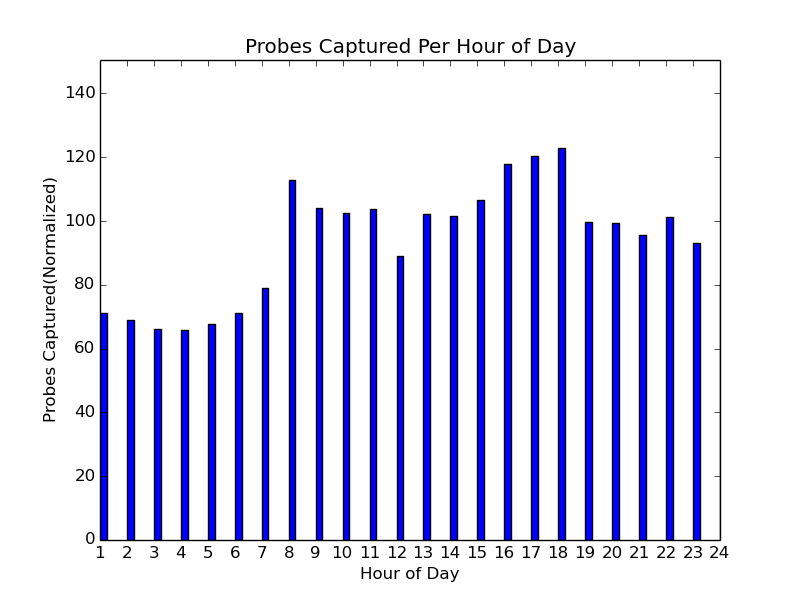
Probes by hour of day

Looking at the number of probes per hour of the day is much more interesting. This is a histogram where the bin width is an hour. I chose to normalize the height of each tally by the number of days included in it. This enables the absolute height of each tally to be compared across all three graphs, even though each one does not include the same number of days.

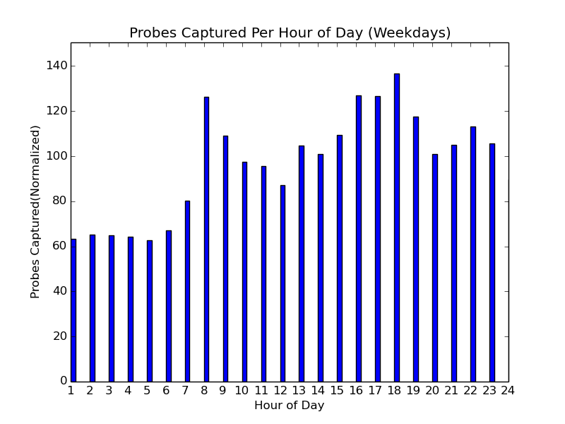
The second graph showing the probes per hour of the weekday is the most striking. It lines up with the idea that traffic peaks in the morning when people are travelling to work and in the afternoon when they are coming home. There is a school bus stop near my house. I'm guessing most school students also carry a cell phone, which might explain the afternoon values beginning to rise earlier than expected.

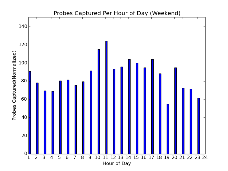
The graph for the weekend shows a strong difference between the weekday graph with activity peaking in the middle of the day.

Stations Per SSID

The next thing I thought would be interesting would be to see how many SSIDs are shared in common by the stations observed. The first question is how many SSIDs have more than one station probing for them.

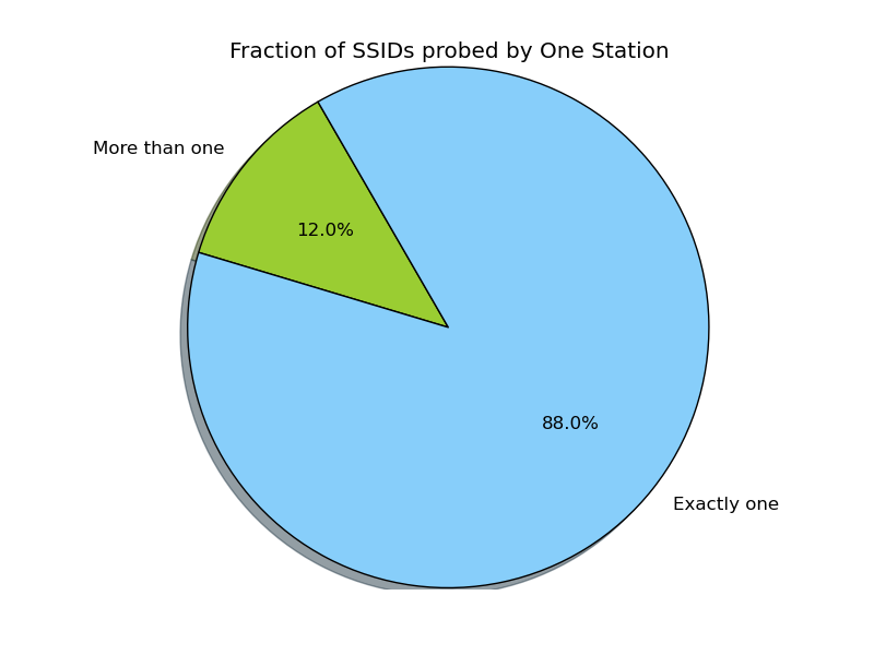
Only 12% of the SSIDs observed had more than one station probing for them. I needed to cut down that part of the dataset even more, so I graphed just the upper quartile.

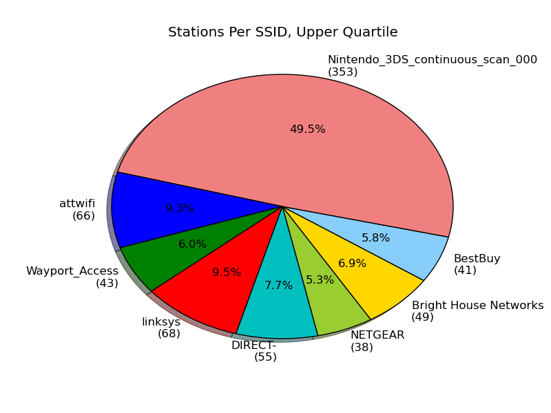
Each SSID is shown along with the number of stations probing for it. Most of these do not stand out very much. "Bright House Networks" is the name of a regional cable provider. "Wayport_Access" is a provider of internet access at McDonald's.

But what exactly is "Nintendo_3DS_continous_scan_000"? It turns out to be something called StreetPass for the Nintendo 3DS. It is used by the handheld to connect to other handhelds. A good explanation of the WiFi component is found here. The handheld uses these probes as a way to announce its presence and set up what amounts to an ad hoc network. The fact that I saw 353 Nintendo 3DS handhelds is surprising to me.

I have not yet figured out what an SSID of "DIRECT-" corresponds to.

The SSID "attwifi" apparently is used by AT&T to offer wireless service to its customers in public places. Interestingly, it seems that some iPhones attempt to connect to this network even if the user does not instruct them to. This phenomenon is detailed here and here. This makes a great target for a man in the middle attack on iOS devices.

The SSIDs "linksys" and "NETGEAR" are the defaults on many home access points.

Where to go from here

At the moment, I'm sitting on this project. I believe that capturing the undirected probes will give me a much more interesting dataset.

While I was working on ideas for the background subtraction, it dawned on me that you could use the observations to measure wait time in a queue. If I had clear view of a traffic light, this would be a really neat application. Unfortunately I do not at this time.

The first 3 digits of each stations MAC address are assigned by the IEEE to specific manufacturers. Due to this, I essentially have access to a popularity map of device manufacturers. I am not sure what I will do with this at this time, but I think there are some interesting possibilities.

Source code

I have updated the project on GitHub with the latest source code. I used the matplotlib python module to generate the graphs.